metacausal.plots.forest

metacausal.plots.forest(boot_result, *, ax=None, order='value', ensemble_label='Ensemble', show_zero=True)

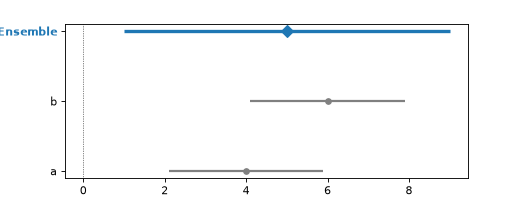
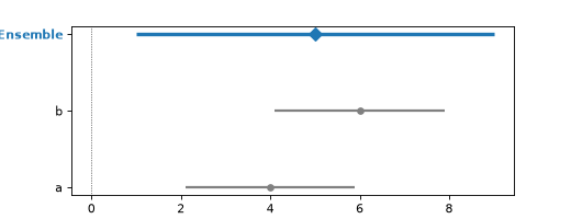
Forest plot of per-component and ensemble ATEs.

Each component row shows the bootstrap mean ATE and its 1 - alpha CI (lower/upper bounds from percentiles of component_boot_ates[name]). The ensemble row uses boot_result.ate and boot_result.ate_ci_{lower,upper} and is always drawn at the top of the plot.

Parameters:

• boot_result (BootstrapResult) – Output of CausalEnsemble.bootstrap(...). Must have a non-empty component_boot_ates mapping.

• ax (Axes | None) – Existing axes to draw on. If None, a new figure is created.

• order (Literal['value', 'alpha', 'ci_width', 'input']) –

  Row ordering for component rows (top-down):

  • "value" (default): ascending bootstrap-mean ATE.

  • "alpha": alphabetical by component name.

  • "ci_width": ascending CI width.

  • "input": insertion order of component_boot_ates.

• ensemble_label (str) – Y-tick label for the ensemble row.

• show_zero (bool) – If True, draw a dotted vertical reference line at ATE = 0.

Returns:

Axes – The axes the plot was drawn on.

Raises:

ValueError – If boot_result.component_boot_ates is empty.

Return type:

Axes

Examples

Works directly on a standalone BootstrapResult (as returned by CausalEnsemble.bootstrap(...)), constructed by hand here with toy bootstrap distributions for two components:

>>> import numpy as np
>>> from metacausal.aggregation import BootstrapResult
>>> from metacausal.plots import forest
>>> boot = BootstrapResult(
...     ate=5.0, ate_ci_lower=1.0, ate_ci_upper=9.0,
...     boot_ates=np.array([3.0, 5.0, 7.0]),
...     cate=None, cate_ci_lower=None, cate_ci_upper=None,
...     component_boot_ates={
...         "a": np.array([2.0, 4.0, 6.0]),
...         "b": np.array([4.0, 6.0, 8.0]),
...     },
... )
>>> ax = forest(boot)
>>> ax.get_xlabel()
'ATE'

(Source code, png)